Best Fit Functions
- Details
- Last Updated: Thursday, 19 November 2020 23:15
- Published: Sunday, 18 October 2020 16:14
- Hits: 1311
Linear Functions:
Before we look into best fit functions, let's look at linear functions. Linear functions are functions that satisfy these 2 requirements:
1. f(a*x) = a*f(x)
2. f(x+y) = f(x) + f(y)
These 2 requirements can be combined into one as f(a*x+b*y) = a*f(x)+b*f(y)
Linear functions are important as they state that any scaling and summation of linear functions is also linear and can be computed easily be separating the terms out. The single order polynomial f(x)=m*x+b is a linear function, while polynomials of higher order as f(x) = a*x^2 + b*x + c aren't. But not all functions which look like linear are linear. We'll see examples below.
Best Fit Functions:
AI is all about finding a best fit function for any set of data. We saw in earlier article that for Logistic Regression, sigmoid sunction is a good function for best fit. However there is nothing special about a sigmoid function. From Fourier theorem, we know that a sum of sine/cosine functions can represent any function f(x) (with some limitations, but we'll ignore those). In fact, any function f(x) can be represented as infinite summation of polynomials of x (again with some limitations, but we'll ignore those). Sine/Cosine functions can also be represented as infinite summation of polynomials of x, so they are also able to represent any function f(x). Since any function can be rep as polynomial of x (Taylor's theorem), that implies that any function f(x) can be represented as summation of any other function g(x) that can be represented as infinite summation of polynomials. .
What about functions g(x) that are not infinite summation of x. Let's say g(x)=4+2*x. Will g(x) be able to represent any function f(x)? Since any func f(x) is infinite summation of polynomials, it can be approximated as finite sum of polynomials too. Of course, lower the number of polynomials terms we have in summation of f(x), less will be the accuracy in representing x. Let's see this with an example:
ex: f(x) = 3 + 7*x + 4*x^2 + 9*x^3 + .....
If g(x) = 4+2*x, then we can write f(x) = A*g(x). If we choose A=3, then then 3*g(x)=12+6*x, which is able to approximate f(x) though not exactly. Not only the higher powers of x are missing, but even the 1st 2 terms for f(x) don't match exactly with A*g(x). No matter how many linear combination of g(x) we use, we can't match the 1st 2 terms of f(x).
i.e f(x) = A1*g(x) + A2*g(x) = (A1+A2)*g(x), which is the same as B*g(x). So, we don't achieve anything better by summing the same function g(x) with different coefficients.
However, if we define 2 linear functions, g1(x) and g2(x), where g1(x)=4+2*x, while g2(x)=1+3*x, then A1*g1(x) + A2*g2(x) can be made to represent 3+7*x, by choosing A1=1/5, A2=11/5. Thus we are able to match 1st 2 terms of f(x) exactly.
However, if we had flexibility in choosing g(x), then we would choose g(x)=3+7*x. Then the 1st 2 terms of f(x) would match exactly with g(x), by using just 1 func g(x)
Similarly, if g(x) is chosen to be 2nd degree polynomial, i.e g(x)=1+2*x+3*x^2, then we can choose g1(x), g2(x), g3(x) to be 3 different 2nd degree poly eqn, and approximate f(x)=A1*g1(x) + A2*g2(x) + A3*g3(x). Or if we had flexibility in choosing g(x), then we would choose g(x)=3+7*x+4*x^2. Then the 1st 3 terms of f(x) would match exactly with g(x).
Continuing the same way, higher the order of g(x), closer will the approximation of f(x) with linear summation of any function g(x).
X as a multi dimensional vector:
Now let's consider eqn in n dimension, where f(x) is not a eqn in single var "x", but in "n" var x1,x2,...xn. i.e we define f(X) where X=(x1 x2 x3 .... xn).
Let's stick to 1st degree linear eqn g(x)=m*x+c. We define g1(x1)=m1*x1+c1, g2(x2)=m2*x2+c2, .... gn(xn)=mn*xn+cn
Then f(x1,x2,...,xn) = g1(x1)+g2(x2)+...+gn(xn) = m1*x1+c1 + m2*x2+c2 + .... mn*xn+cn = m1*x1 + m2*x2 + ... mn*xn + (c1 + c2 + ... + cn) = m1*x1 + m2*x2 + ... mn*xn + b (where b = c1+c2+...+cn)
So, for n dimensional space, if we choose g(x1,x2,...,xn) = m1*x1 + m2*x2 + ... mn*xn + b, then we can get a best fit n dimensional plane to function f(x1,x2,...,xn). However, the approximation function is 1st degree polynomial, so it doesn't have any curves or bends (just flat plane). This is a linear function.
Linear function with bendings:
What if we are able to introduce a bend in linear function g(x), so that it's not a straight line anymore. If we then add up these functions with bends, we can have any kind of bend desired at any point. Then we may be able to approximate any function f(x) with these function g(x) by having a lot of these g(x) functions with bends.
Let's see this in 3D, since multidimensional is difficult to visualize. We write above f(x) in 2D as:
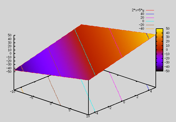
f(x,y)=m1*x + m2*y = 2*x+5*y
gnuplot> splot 2*x+5*y => As seen below, this plot is a plane
Now, we take a simple function called absolute function. It has a bend, and slopes of 2 lines for x<0 and x>0 are -ve of each other.
gnuplot> splot abs(x) => As seen below, this plot has a bend at x=0

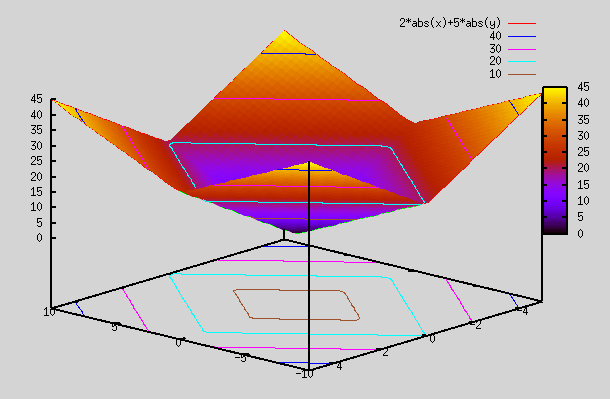
Now, we plot the same function as first one, but this time with abs functions applied to x and y. As you can see, we have bends so that we can generate planes at different angles to fit complex curves.
gnuplot> splot 2*abs(x)+5*abs(y)
Is abs() function linear? It does look linear, but it has a bend (so 2 linear functions in 2 range).
Let's pick 2 points: x1=1 and x2=-1. Then abs(x1+x2) = abs(1-1) = abs(0) = 0. However, if we compute f(x1) and f(x2), we get f(-1)=1, and abs(1)=1. So. abs(x1)+abs(x2) = 2 which is not same as abs(x1+x2). So, abs() function is not linear. Similarly any 1st order eqn with a bend is not linear.
Taylor theorem tells us that any function can be expanded into infinite polynomial series. We should be able to find Taylor series for abs(x) function.
Note: f(x) = abs(x) = √(x^2) = √(1+(x^2 - 1)) = √(1+t) where t = (x^2 - 1)
√(1+t) is a binomial series which can be expanded into Taylor series as explained here: https://en.wikipedia.org/wiki/Binomial_series#Convergence
(1+t)^1/2 = 1 + (1/2)t - (1/(2*4))t^2 + ((1*3)/(2*4*6))t^3 - ...
So, f(x) = abs(x) = 1 + (x^2-1)/2 - (1/(2*4))(x^2-1)^2 + ((1*3)/(2*4*6))(x^2-1)^3 - ... = [1-1/2-1/(2*4)-...] + x^2*[1/2+1/4+...] + x^4*[-1/(2*4)+....] + x^6*[...] + ...
Thus we see that we get Taylor series expansion of abs(x) as summation of even powers of x. So, it is indeed not a linear eqn. As it's infinite summation, it can be used to represent any function as explained at top of this article.
ReLU function:
Just as absolute func has a bend and is not linear, many other linear looking functions can be formed which have a bend, but are not linear. One such function that is very popular in AI is ReLU (Rectified linear unit). Here instead of having slope as -1 for x<0, we make the slope=0 for x<0. This function is defined as below:
Relu(x) = x for x>0, = 0 for x<0
gnuplot> f2(x)=(x>0) ? x : 0 #this is the eqn to get a ReLu func in gnuplot
gnuplot> splot f2(x)
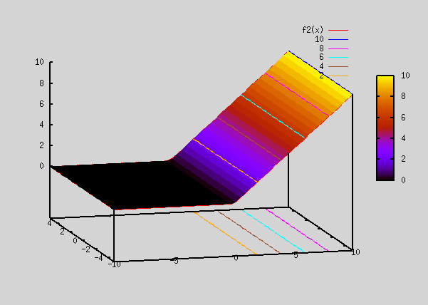
The above plot looks similar to how abs(x) function looked like, except that it's 0 for all x <0.
Now, let's plot a function which is a difference of the 2 Relu plots.
gnuplot> splot f2(x+5)-f2(x-5)
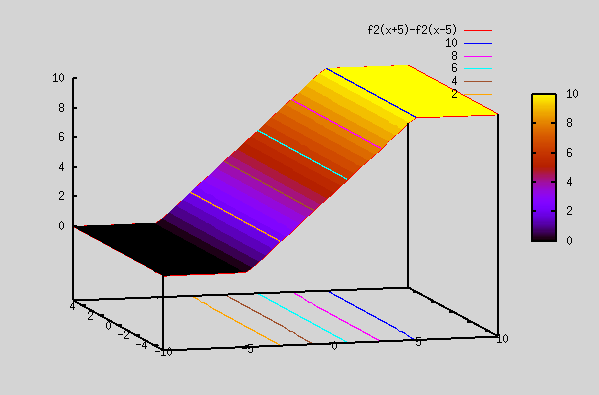
The Relu plot above ( Relu(x+5) - Relu(x-5) ) now has 2 knees at x=-5 and x=+5. It actually resembles a sigmoid function (explained below). However, it doesn't have smooth edges as in sigmoid func. Since sigmoid function can fit any func, linear sum of Relu func can also fit any func. The advantage with Relu is that it's similar to linear (it's linear in 2 separate regions, although it's not linear overall), so derivatives are straight forward.
There is very good link here on why Relu functions work so well in curve fitting (and how are they non-linear inspite of giving an impression of a linear eqn):
Sigmoid function:
Sigmoid function being an exponential function, it's has higher powers of x in it's expansion, instead of just having "x" (i.e x, x^2, x^3, etc).
i.e σ(z) = 1 / (1 - e^(-z)) = A1 + A2*z + A3*z^2 + ... (taylor expansion)
Sigmoid function would fit better than Relu functions above as they have higher orders of x (so they have smooth edges). However, the are also more compute intensive, and so are not used except when absolutely necessary.
Let's plot a 2D sigmoid funcion, where z=a*x+b*y. We use gnuplot to plot the functions below:
f1(x,y,a,b)=1/(1+exp(-(a*x+b*y)))
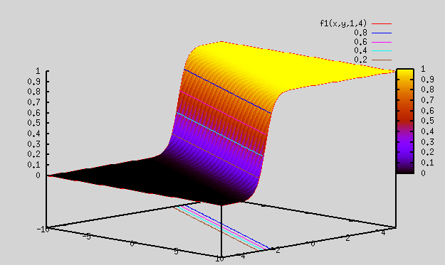
Plot 0:
gnuplot> splot f1(x,y,1,4) => As seen below, this is a smooth function varying from 0 to 1. Looks kind of similar to difference of Relu function plotted above.
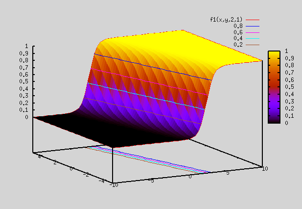
Plot 1:
gnuplot> splot f1(x,y,2,1) => As seen below, plot is same as that above, except that the slope direction is different
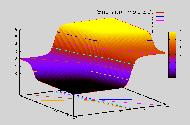
Plot 2:
gnuplot> splot (2*f1(x,y,1,4) + 4*f1(x,y,2,1)) => Here we multiply the above 2 plots by different weights and add them up. So, resulting plot is no longer b/w 0 and 1, but varies from 0 to 6.
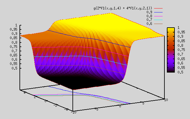
We define another sigmoid function, which is in 1 dimension
g(x) = 1/(1+exp(-(x)))
Plot 3:
gnuplot> splot g(2*f1(x,y,1,4) + 4*f1(x,y,2,1)) => Here we took sigmoid of above plot, so resulting plot is confined to be b/w 0 and 1. However, because of the weights we chose, resulting plot ranges from 0.5 to 1, instead of ranging from 0 to 1.
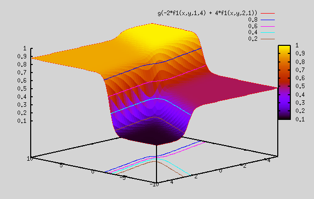
Plot 4:
gnuplot> splot g(-2*f1(x,y,1,4) + 4*f1(x,y,2,1)) => almost same plot as above, except that z range here is from 0.1 to 1 (by changing weight to -ve number)
Summary:
Now, that we know Relu and sigmoid functions are not linear, and in fact are polynomials of higher degree. As such, they can be used to represent any function, by using enough linear combinations of these functions. So, they can be used as fitting functions to fit any n dimensional function. These are used very frequently in AI to fit our training data. We will look at their implementation in AI section.