Calculus
- Details
- Last Updated: Sunday, 12 April 2026 18:14
- Published: Tuesday, 03 June 2025 01:29
- Hits: 1100
Calculus:
We'll start with limits and then move to differentials and integrals.
Best website for all Calculus notes =>
- Calculus 1 => https://tutorial.math.lamar.edu/Classes/CalcI/CalcI.aspx
- Calculus 2 => https://tutorial.math.lamar.edu/Classes/CalcII/CalcII.aspx
- Calculus 3 => https://tutorial.math.lamar.edu/Classes/CalcIII/CalcIII.aspx (much more advanced topics on 3D integral, partial derivatives, multiple integrals, etc)
- Differential Eqn => https://tutorial.math.lamar.edu/Classes/DE/DE.aspx (1st year college maths)
Nice cheat sheet showing all imp Calculus formulas => https://math.colorado.edu/math2300/resources/calc1/lamar/Calculus_Cheat_Sheet_All.pdf
Limits:
Limits are one of the easiest to master. They form the basis of calculus. When we say limit, we are trying to find the value of a function, as it approaches a particular value of a variable.
ex; Y= 2*x+5. This is a straight line, and when I say what is the value of Y at x=3, it's 2*3+5=11. No if I say, what's valve of Y as x approaches 3 from left side of graph (denoted as -> 3-), or from right side of graph (denoted as -> 3+), it's still 11. So, most of the cases limit is as simple just substituting the value.
In some, the exact value of the Func doesn't exist at that point, but in this case, limit may still exist, since Limit says it approaches that value, but is never exactly that value.
ex: Y = (x^2-4)/(x-2). Here at x=2, the function is 0/0 which is undefined. However, we can write it as Y=(x-2)(x+2)/(x-2). If x≠2, then we can cancel out (x-2) from top and bottom, and func Y=(x+2). Now as x->2 (from left or right, doesn't matter), the value is 4. However, at exactly x=2, the value doesn't exist (you mark it as a open dot instead of a filled in dot). Since the value of limit (=4) is same both from left and right, we say that the limit exists, even though the limits don't give the same value of 4 at x=2, i.e Y(x=2)≠4.
When evaluating limits, Func which yield values as 0/0, ∞/∞, 0*∞ are all undefined, and hence you have to either cancel out some term, or rewrite the expression so that it can be evaluated to a known value on substitution (and NOT yield undefined values). Most of the complicated function limits are evaluated by expanding the complex function as Taylor series (i.e as polynomial function). Then something usually cancels out leading to a limit value.
Some well known limits are:
- Lt x->0 (sin(x))/x = 1 (write sin(x) as Taylor series and cancel out x from numerator and denominator). It's 0/0, but evaluates to 1 in limiting case. On Khan academy, proof of this is provided using other limit theorem (sandwich theorem of limits), which finds the limit of 2 other functions, and sandwiches this func b/w those 2 func. Since the limit of other 2 func approaches 1, the limit of this func will also need to be 1.
- Lt x->0 (1-cos(x))/x = 0 (expand using Taylor series). It's 0/0, but evaluates to 0 in limiting case (unlike sin case above which evaluates to 1).
- Lt x->∞ (1+1/x)^x = e. Here inside term goes to 0 while exponent term goes to ∞, so hard to see it can approach a particular value as e. Can be proved by doing "Binomial Thm (BT)" expansion of series, or by taking log of this func, and then using limit of log. One such proof using BT => https://www.mathdoubts.com/lim-1-plus-1-by-x-whole-power-x-as-x-approaches-infinity-proof/
- More limits => https://planetmath.org/ListOfCommonLimits
ex: Limit of sin(x))/x can easily be found by using L'Hôpital's Rule. Lt x->0 (sin(x))/x = Lt x->0 (cos(x))/1 = 1/1 = 1.
Differentiation (Derivatives):
Differentiation follows from limits. A derivative of a function is the slope of a function at every point of the function. The slope at a point is defined as a line that touches the function at only 1 point (i.e a tangent at that point). This slope itself may be another function, and it's denoted as f´(x) (i.e f with a prime on top).
Avg slope of a function b/w any 2 points x1 and x2 is = [f(x2)-f(x1)] / (x2-x1). Now if we start getting x2 closer to x1, then avg slope we get is for a narrower section of the function. If we make x2 infinitesimally close to x1, then, in the limiting case, we get the slope of the function at the point x1.
Let's rewrite x2 as x2=x1+Δx, then slope = [f(x1+Δx) - f(x)] / Δx
So, f´(x) = Lt Δx->0 [f(x+Δx) - f(x)] / Δx => The eqn we get for derivative is the function that shows the slope of f(x) at any point x. The limit has to exist from both left and right side and be the same, only then f´(x) exists and it's value is the common value. Only in this case is the function f(x) said to be differentiable.
Conditions for differentiability at a point c:
- Func needs to be continuous at point c (in this case, limit will be same on both sides of point c, and equal the value of func at c, i,e f(x=c) = Limits from both left and right.
- Func needs to have same slope on both sides (i.e no sharp turns or infinite slope).
Conditions for differentiability (with nice examples) => https://math.libretexts.org/Courses/Irvine_Valley_College/Math_3AC%3A_Analytic_Geometry_and_Calculus_I/07%3A_Derivatives/7.04%3A__Differentiability
ex: f(x)=x^2, find f´(x). Here we find derivative using the defn above.
f´(x) = Lt Δx->0 [f(x+Δx) - f(x)] / Δx = Lt Δx->0 [(x+Δx)^2 - x^2] / Δx = Lt Δx->0 [2.x.Δx + Δx^2]/Δx = Lt Δx->0 [Δx(2.x+Δx)] / Δx = Lt Δx->0 2.x+Δx = 2.x
So, slope of function x^2 is 2.x at any point x. We can verify this by drawing slopes at x=1, x=2, x=4, etc and confirm that the slope is indeed 2, 4, 8, which is 2.x !!
Similarly derivatives can be found for many common functions. In most cases, we have to do a Taylor series expansion to cancel out Δx in both numerator and denominator.
f(x)=sin(x). To find f´(x), we expand sin(x) as Taylor series,, cancel out Δx, and the series left is cos(x). So, f´(x) = cos(x)
If f(x)=cos(x), then f'(x) = -sin(x)
Cheat sheet => https://tutorial.math.lamar.edu/pdf/calculus_cheat_sheet_derivatives.pdf
Derivative Rules:
- Constant Multiple Rule: d/dx[k*f(x)] = k* d/dx(f(x)), where k is a constant.
- Power rule: d/dx(x^n) = n*x^(n-1). Most widely used to differentiate polynomials. Any continuous function can be written as a polynomial, so individual terms of the polynomial can be differentiated using this formula. If we keep on differentiating poly of x^n n times, then it will keep reducing the power of poly func by 1 each time, and ultimately the result would be 0.
- Sum/Difference Rule: d/dx [f(x) + g(x)] dx = d/dx[f(x)] + d/dx[g(x)] (instead of +, we can have - too)
- Product rule: d/dx [f(x).g(x)] = g(x).d/dx(f(x) + f(x).d/dx(g(x) => basically you differentiate each function separately and multiply it with the undifferentiated func.
- Quotient Rule: d/dx [f(x)/g(x)] = g(x).d/dx(f(x) - f(x).d/dx(g(x) / [g(x)]^2. This can be derived from product rule as g(x) can be replaced with 1/g(x). Then d/dx(1/g(x)) = -1/[g(x)]^2 * d/dx(g(x)) and we get the quotient rule.
- Chain Rule: Written in 2 forms:
- d/dx [f(g(x))] = d/d(g(x)) [f(g(x))] * d/dx(g(x)) => NOTE: the 1st derivative is wrt g(x) and NOT x. You may substitute g(x) with var "u". That is the form that the 2nd form of chain rule is written in as shown below.
- dy/dx = dy/du * du/dx where y may be written as a func of var u.
Some common derivatives:
Link for common derivatives and rules => https://www.mathsisfun.com/calculus/derivatives-rules.html
- d/dx(e^x) = e^x (drive from defn of derivative, and then using series expansion of e^x).
- d/dx (a^x) = ln(a). a^x. We can derive this from differentiation of e^x. a^x can be rewritten as e^(x ln(a)). This is because if we take natural log of both sides, then ln(a^x) = ln (e^(x ln(a)) => x (ln a) = x (ln a), so both sides become equal. Now d/dx(a^x) = d/dx(e^x(ln a) = e^(x(ln a)) . d/dx(x * ln(a)) = ln (a). e^(x(ln a) = ln(a). a^x.
- d/dx(ln x) = 1/x . Since ln (x) is inverse fn of e^x, we can use above derivative of e^x to find this one. Let y=ln(x) => x=e^y, => d/dx(x) = d/dx(e^y) => 1 = d/dy(e^y).dy/dx => 1=e^y.dy/dx => dy/dx = 1/e^y = 1/x .
- NOTE: ln (x) is only defined for x>0. This will be important in integral (discussed below) as If we want to have ∫ 1/x = ln(x) only for x>0. If x<0 in limits, then we can only do integral only if we take mod x, i.e ln |x|. So ∫ 1/x = ln(|x|) if we want to be exact. This ensures that just as 1/x graph exists in 1st and 3rd quadrant, ln(x) exists in all 4 quadrants for all values of x.
- d/dx(logax) = d/dx(ln(x)/ln(a)) = 1/(x.ln(a)).
- Trignometric func: Differentiation of Trignometric functions require using the limit theorems for basic func as sin(x). Others can be derived using this differentiation.
- Regular trig func: sin, cos, etc
- sin(x) or cos(x) => derivative of cos(x) has -ve sign.
- sin(x): d/dx(sin(x)) = cos(x). Use basic limits as sin(Δx)/Δx =1, and [(1-cos(Δx)]/Δx =0 as Δx approaches 0 to prove the sin(x) derivative. Others follow.
- cos(x): d/dx(cos(x)) = -sin(x). NOTE the -ve sign in derivative.
- cosec(x) or sec(x) =>derivatives that give sin(x) or similar form have -ve sign in final result. So, csc(x) gives -ve sign when differentiating.
- csc(x): d/dx(cosec(x)) = d/dx(1/sin(x)) = [-1/sin2(x)].cos(x) = -cosec(x).cot(x). NOTE the -ve sign in derivative.
- sec(x): Similarly d/dx(sec(x)) = d/dx(1/cos(x)) = [-1/cos2(x)].[-sin(x)] = sec(x).tan(x). NO -ve sign.
- tan(x) or cot(x):
- tan(x) => d/dx(tan(x)) = d/dx((sin(x)/cos(x)). Using quotient rule, we get f'(x)= sec2(x)=1/cos2(x)
- cot(x) => d/dx(cot(x)) = d/dx((cos(x)/sin(x)). Using quotient rule, we get f'(x)= -cosec2(x) = -1/sin2(x). Or other way is by using d/dx(1/f(x)) where f(x)=tan(x). So, d/dx(1/tan(x)) = -1/tan2(x).d/dx(tan(x)) = -1/tan2(x).(1/cos2(x)) = -1/sin2(x). NOTE the -ve sign in derivative.
- sin(x) or cos(x) => derivative of cos(x) has -ve sign.
- Inverse trig func: These are written as sin-1(x) or arcsin(x). For each pair below, the derivative of other inverse func is just a -ve of the other one, so easy to remember.
- sin-1(x) or cos-1(x) => We let sin-1(x) = y => sin(y) =x => cos(y).dy/dx = 1 => dy/dx= 1/cos(y) = 1/[√(1-sin2(y)] = 1/( √(1-x2). Similarly d/dx(cos-1(x)) = -1/sin(y) = -1/[√(1-sin2(y)] = -1/( √(1-x2) (we just add a -ve sign for this). In these x≠+/-1, as that will yield ∞.
- tan-1(x) or cot-1(x) => We let tan-1(x) = y => tan(y) =x => sec2(y).dy/dx = 1 => dy/dx = 1/ sec2(y) = cos2(y) = 1/(1+x2). Similarly d/dx (cot-1(x)) = -1/(1+x2) (we just add a -ve sign for this)
- csc-1(x) or sec-1(x) =>These are less used. We can use similar techniques. d/dx (sec-1(x)) = 1/[|x|.√(x2-1)]. Similarly d/dx (csc-1(x)) = -1/[|x|.√(x2-1)] (we just add a -ve sign for this). In these x≠+/-1, as that will yield ∞. Also, we have to do |x| as without modulus, the slope is incorrect for -ve values of x, so we do |x| to make it correct for both +ve and -ve values of x. One such proof here: https://math.libretexts.org/Bookshelves/Calculus/Supplemental_Modules_(Calculus)/Differential_Calculus/Differential_Calculus_(Seeburger)/Derivatives_of_the_Inverse_Trigonometric_Functions
- Regular trig func: sin, cos, etc
Tricky differentiation using above rules:
- ex: d/dx(x^x). Take y=x^x => ln(y)=xln(x) => d/dx(ln(y)) = d/dx(xln(x)) => 1/y*dy/dx=ln(x) + 1 => dy/dx=y[1+ln(x)] => d/dx(x^x) = x^x * [1+ln(x)]
Derivative of inverse functions:
If we have f(x) and it's inverse g(x)=f-1(x), then if slope of f(x) = m at pt (x1,y1), then slope of g(x) will always be 1/m. Reason being that inverse function is just y replaced by x (and x replaced by y). So if original func f(x) had slope m=Δy/Δx, then it's inverse func g(x) will have slope Δx/Δy (as x and y are interchanged for inverse func), which is = 1/m. So, the g´(x) = 1/f´(x). The only point to watch out is that if the slope of original func f(x) was at point (x1,y1), then the inverted slope is at point (y1,x1) as the x,y coordinates get interchanged. So if f(x) slope is m at (b,a), then g(x) slope will be 1/m at (a,b). => a=f(b) => b=f-1(a)
g´(x=a) = 1/f´(x=b) => g´(x=a) = 1/f´(x=b) => g´(x=a) = 1/f´(g(x=a)) = 1/f´(f-1(x=a)) [since g(x) = f-1(x))]
ex: f(x)=x^2, then g(x)=f-1(x)=√x
f´(x)=2x, g´(x)=1/(2x), At x=3, f´(x)=2x=6 (at coord (3,9)), so g´(x)=1/(2x) = 1/6 at coord (9,3). NOTE: the coordinates chaged. If we want to find g´(x=3) (i.e coord (3,√3)), then we need to find f´(x=√3) = 2√3 => g´(x=3) = 1(2√3)
We can also use above formula directly: g´(x=a) = 1/f´(g(x=a)) => Since g(x=3) = √3, g´(x=3) = 1/2x @x=√3 = 1(2√3), which is same as what we obtained above.
Maxima/Minima:
Derivatives can be used to find maxima and minima if functions. This is one of the most used application of derivatives in real life.
KA: https://www.khanacademy.org/math/ap-calculus-bc/bc-diff-analytical-applications-new/bc-5-8
Following defn used to describe shapes of func when dealing with max/min: NOTE: A "down func" implies real func, while "up func" implies opposite of the real func behaviour. For ex: both "convex" or "convex down" imply a rice bowl kept on table, which is how "convex" func are defined. However a "convex up" func implies the opposite behaviour, i.e a rice bowl kept upside down on table.
- Convex func: (aka Concave upward or convex downward): Any func whose slope increases is convex or concave up (like a rice bowl kept on table), i.e slope goes from -ve to 0 to +ve or any part where slope is increasing.
- Concave func (aka concave downward or convex upward): Any func whose slope decreases is concave or convex up (like a rice bowl kept upside down on table), i.e slope goes from +ve to 0 to -ve or any part where slope is decreasing.
- Infection point: This is the point where the func changes from convex to concave or vice versa.
A continuous and smooth function (most of the real functions are smooth, an exception is absolute value func) will have it's slope=0 at maxima and minima. These are local max/min, as many of these local max/min may exist. There's no way known to find the absolute max/min of any func. Over a limited domain of x values (i.e x goes from x1 to x2), we can determine absolute max/min by looking at all points where slope is 0, undefined or at end points. Whether the point is maxima or minima is determined by 2nd derivative.
- 1st derivative: Given f(x), find first derivative f'(x). If f'(x) =0 at x=x1, it's either a maxima, a minima or a infection point. An infection point is a point where slope is 0, but instead of reversing direction (i.e slope), it keeps on moving in same direction.
- 2nd derivative: Now find 2nd derivative f''(x) at x=x1. Depending on 2nd derivative sign, we can determine whether it's max or min
- Maxima: If f''(x1) < 0, then x1 is a point of local maxima. This is because, at maxima, it's concave, so slope of this func goes from +ve to -ve (decreasing). Then, derivative of this slope (i.e f''(x)) will be -ve. If you don't want to check for 2nd derivative, then you can also check sign of first derivative, f'(x). If f'(x) changes sign from +ve to -ve when going thru x1, then it's a maxima.
- Minima: If f''(x1) > 0, then x1 is a point of local minima. This is because, at minima, it's convex, so slope of this func goes from -ve to +ve (increasing). Then, derivative of this slope (i.e f''(x)) will be +ve. If you don't want to check for 2nd derivative, then you can also check sign of first derivative, f'(x). If f'(x) changes sign from -ve to +ve when going thru x1, then it's a minima.
- Infection point: Here, func changes from convex to concave or vice versa, implying f''(x) changes sign from +ve to -ve or vice versa. Basically f''(x)=0 at point of infection (as sign change can only happen when it passes thru 0). At infection point, slope of the original func, f(x), may or may not be 0 (i.e f'(x)=0 or f'(x)≠0).
- If f'x(0)=0 and f''(x)=0, then func continues going in same dirn after hitting a flat portion. No max or min exists, though slope of f(x) does go to 0
- If f'x(0)≠0 and f''(x)=0, then func is changing shape from convex to concave or vice versa. No max or min exists as slope of f(x) never goes to 0
Plotting functions: Complicated functions can be plotted by utilizing calculus. We find derivatives to find out where the slope is 0 or undefined, as well as the regions of increasing/decreasing value, which helps us plot it. 3 different kinf of func really easy to plot using calculus. See in KA for these examples:
- Polynomial functions: Ex: f(x)= 3x^4-4x^3+2. f'(x) =0 at x=0,1. Now, we find f''(0) and f''(1). If it's > 0, then it's min, else it's max. At x=0, f''(0)=0, implying it's infection point, so slope remains same. to find whether func is inc or dec.
- Log function: Ex: f(x)=
Integration (Integral):
Integration is inverse of differentiation. Integral is the inverse function of derivative. We denote it as ∫ f(x). Given function f(x), if F´(x) = f(x), then ∫ f(x) = F(x). F(x) (denoted with capital F) is the inverse func of f(x). See Inverse function in other sections.
F(x) -> differentiate -> f(x). F´(x) = f(x),
F(x) <- integrate <- f(x). F(x) = ∫ f(x).
Integration was originally developed as "finding area under curve". Later Barlow and Toricelli in 17th century found hints of connection b/w differentiation and integral. Barrow provided the 1st proof of "fundamental Thm of Calculus". Later Newton and Leibniz did more advanced work on calculus, where integral was found to be inverse function of differentiation, which made it easy to solve integral
But why is integration area under a curve? Let's say A(x) is some function of f(x). At x=x1, A(x) is A(x1). Now, if we take incremental "dx" at x=x1, and compute f(x).dx, then f(x).dx gives area of the incremental rectangle formed. So, incremental increase in area is f(x).dx. So, A(x) must be the area of the function, as incremental area dA(x)=f(x).dx => dA(x)/dx = f(x). Or A(x) = ∫ f(x).dx
This vid shows it formally by using MVT => https://www.youtube.com/watch?v=U3u0PF7n-xg
Integration is usually taught as avg value of a continuous func. To make it easier, we divide f(x) into N discrete sections and then find avg value.
Then avg = [∑f(x) ] / N, where summation is over N points, and each point is spaced apart by dx, so no. of points N = (b-a)/dx. So, area = Avg height of f(x) * base = [∑f(x) ] / (b-a) * dx * (b-a) = [∑f(x) ] * dx where a,b are endpoints on x axis
Now if we start taking limit dx->0, then avg value of this func approaches closer to it's real value. So, Area = Limit dx->0 [∑f(x) ] * dx = b
a∫ f(x).dx
Reimann Integral (RI): This is the discrete version of integrals, where we divide the area under curve into smaller rectangles, and then sum all the rectangles.
Area of f(x) from x=a to x=b => Divide into n rectangles, where width of each rect is same and = (b-a)/n. Then Area of all rectangles = xi=b
xi=a∑[(b-a)/n *f(xi)] = k=n
k=0∑[(b-a)/n *f(a + (b-a)*k/n)] . Writing func in this form gets the right lower and upper limit as f(k=0) = f(a + (b-a)*0/n) = f(a) and f(k=n) = f(a+(b-a)*n/n) = f(b).
Now to get exact area, the number of rectangles should -> infinity, i.e n-> ∞. So, RI = Limit n->∞ k=n
k=0∑[(b-a)/n *f(a + (b-a)*k/n)]
ex: RI rep of b=6
a=2∫ √xdx = Limit n->∞ k=n
k=0∑[(b-a)/n *f(a + (b-a)*k/n)] = Limit n->∞ k=n
k=0∑[4/n *f(2 + 4*k/n)] = Limit n->∞ k=n
k=0∑[4/n *√(2 + 4*k/n)]
Fundamental Thm of Calculus (FTC):
There are 2 parts to fundamental thm of calculus. They connect differentiation and indefinite integration to each other. Part 1 is used to find the derivative of an integral whereas Part 2 is used to evaluate a definite integral. Both are proved here => https://www.cuemath.com/calculus/fundamental-theorem-of-calculus/
1st FTC: This connects diff and integration. For a continuous function f(x) on an interval [a, b] with the integral: F(x) = x
a∫ f(t).dt , then the derivative of the integral F(x) gets us the original function f(x) back again, i.e F'(x)= f(x). Stated differently, derivative of the integral of f with respect to its upper limit (which is a variable) is the function f itself.
ex: f(x)=2x. Then F(2x^3) = 2x^3
a∫ f(t).dt = 2x^3
a∫ 2t.dt = (2x^3)^2-a^2. Take z=2x^3 => F'(z)=2z which is same as f(z). If we want to find d/dx [ 2x^3
a∫ f(t).dt ], then choosing z=2x^3 and using 1st FTC, we get d/dz [ z
a∫ f(t).dt ] * dz/dx = f(z)*d/dx [2x^3] = 2z*6x^2 = 2(2x^3)*6x^2 = 24x^5. If the lower limit is variable and upper limit is const, then we use the -ve property to make the upper limit variable, i.e a
x∫ f(t).dt = - x
a∫ f(t).dt
2nd FTC: This helps in finding definite integral, so that we don't need to use Reimann summation to find area under a curve. When we have a continuous function f(x) on an interval [a, b], and its indefinite integral is F(x), then b
a∫ f(x).dx = F(b) - F(a) where F´(x) = f(x).
There are 2 FTC, but they are generally mentioned as one with 2 parts (strictly there are 2 FTC, but 1st FTC is kind of assumed). What's insane is that the area of the whole curve can be found by just looking at the values of antiderivative at the endpoints of the curve !! We'll see why that happens below.
Essence of Calculus explaining Integration as area under curve => https://www.3blue1brown.com/lessons/integration
We learn integration as the area under the curve. However, the function that we get via integration F(x) is actually the inverse function of f(x), i.e F´(x) = f(x). But differentiation gives the slope, while it's inverse func gives the area. How is the slope and area related? This fundamental question is explained nicely here => https://www.3blue1brown.com/lessons/area-and-slope
To see this relationship, 2 key points to observe:
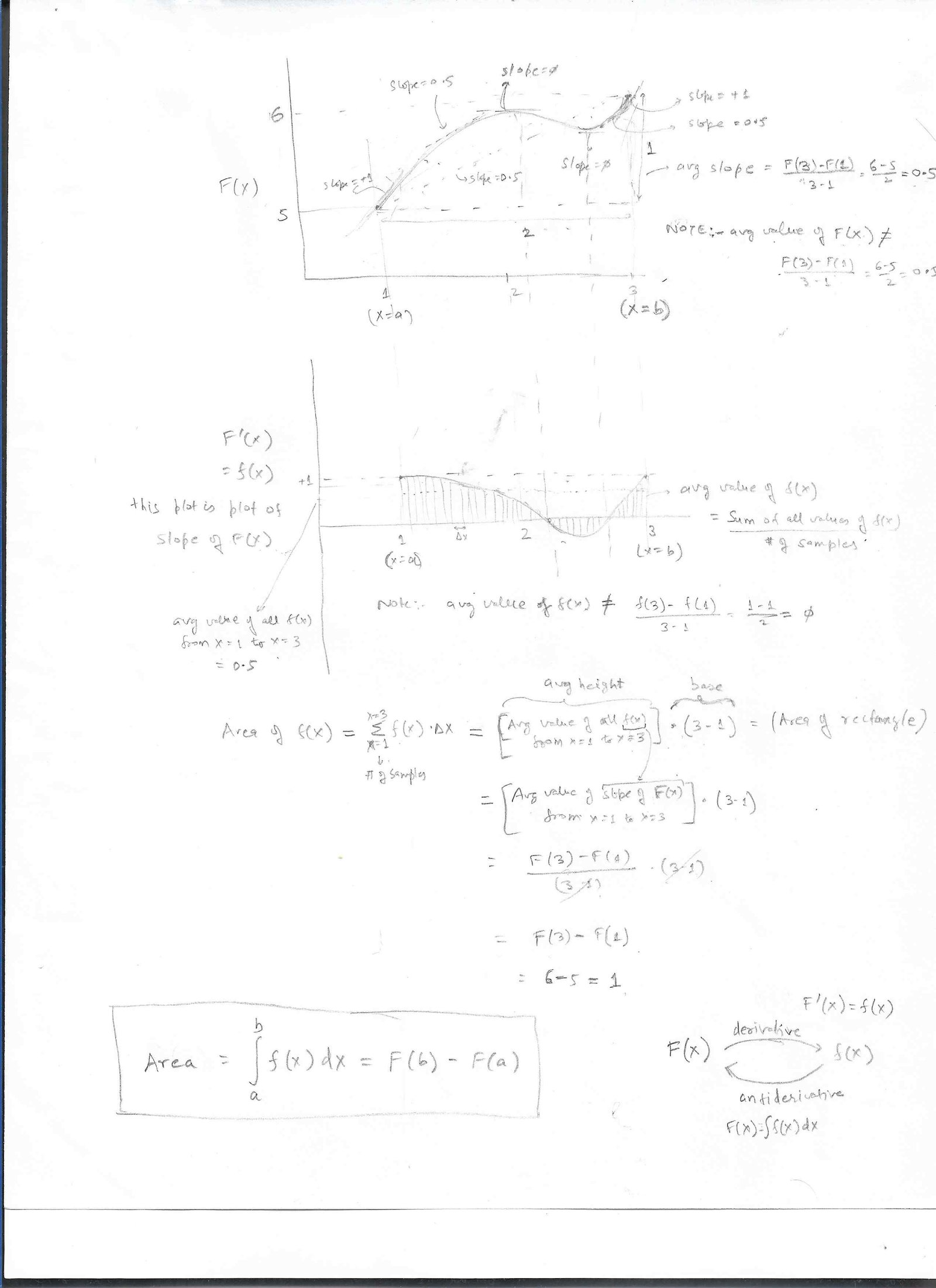
- Avg slope for any func can be calculated by just looking at End Points: If you were given a bunch of numbers in any order, would you be able to calculate it's avg just by looking at 1st and last number? Answer is => NO. You won't be as the avg is decided by all the numbers. Now consider continuous plot of such numbers. Again, it's the same thing => you won't be able to calculate the avg of this continuous func, just by looking at the 2 endpoints of the curve. But now, let's say, I calculate the slope of this function, and plot this new function which is the slope of our original function at every point of the graph. Can I calculate the avg of this slope function, by just looking a the 2 endpoints? Surprisingly, you can now. Why does this happen. Because, with slope, if the slope goes up a certain magnitude above the avg, the slope has to come down the same magnitude below the avg, to give us the avg. It also follows from Mean Value Thm and from intuition. So, the jist is => The avg slope (rate of change of Y wrt X) of any function could be found by just looking at the 2 endpoints.
- Area of a function: it can be calc as avg height of func multiplied by the width of the base. The avg slope of any func as seen above = [F(b)-F(a)]/(b-a), where a,b are endpoints on x axis. If we plot the slope function (i.e a function f(x) that is the slope of F(x) for all points on x axis), then the area of f(x) will be = Avg height of f(x) * base. But avg height of f(x) = avg slope of F(x) (as f(x) is slope func of F(x)). Since avg slope of F(x) = [F(b)-F(a)]/(b-a), that's the avg height of f(x). So, area of f(x) = avg height of f(x) * base = [F(b)-F(a)]/(b-a) * (b-a) = [F(b)-F(a), which proves the theorem.
Diagram showing proof of Fundamental Thm of Calculus
Finding area of a curve:
As we saw above, We use this formula for area under a curve from x axis (Y=0) to the function f(x): Area = b
a∫ f(x).dx = b
a∫ y.dx (since f(x)=y). Other way to find area is to rotate the paper 90 degrees anticlockwise and then integrate with dy, i.e Area = f(b)
f(a)∫ x.dy Here limits a and b change to f(a) and f(b), since we are integrating along Y-axis. This gives the area of the remaining portion of the rectangle bounded by a, b, f(a), f(b). If we add up the 2 area, we should get the area of the rectangle minus the smaller rectangle = [b*f(b)) - a*f(a)].
ex: y=x^2. Area from x=1 to x=3 is b=3
a=1∫ y.dx = b=3
a=1∫ x^2.dx = [x^3/3] from x=1 to x=3 => 1/3[3^3-1] = 26/3.
Now we take area along y axis. Then x=√y. Limits are y=3^2=9, 1^2=1. So, area from y=1 to y=9 is b=9
a=1∫ x.dy = b=9
a=1∫ √y dy = 2/3* [y^3/2] from y=1 to y=9 => 2/3[9^3/2-1] = (26*2)/3.
The area of the rectangle formed is (3*9)-(1*1) = 27-1 = 26, which is the sum of 26/3+26*2/3=26.
NOTE: Area of the figure under the X-axis is calculated as -ve while area above the x-axis is calc as +ve (automatically happens the way we integrate). If we want to find the absolute area, then we have to find the area of the regions separately and then add the absolute values of the 2 area.
Finding arc length of a curve:
To find the arc length, we use pythagoras thm in calculus.
Any length Δl2 = Δx2 + Δy2 => Total length of arc from x=a to x=b is [∑Δl ] = [∑√ ( Δx2 + Δy2) ] = ∑[√ ( 1 + Δy2/Δx2 ) * Δx] = b
a∫ √ ( 1 + dy2/dx2 ) ] * dx (by converting to integral) = b
a∫ √ ( 1 + f’(x)2 ) dx
FIXME: Why does this not work (it's missing sq root)? 2Δldl/dx = 2Δx + 2Δydy/dx => 2dl/dx = 2 + 2dy/dx (differentiating both sides wrt dx) => dl/dx = 1 + f’(x)
Finding Volume under a curve:
Generally for finding volume, surface area, etc, we need to use 2D calculus (involving both var dx and dy). But many times, these 3D figures are symmetric, and we are able to generate the 3D figures from the 2D figure by making concentric circles, etc. Then we can find volume or surface area by just using single variable, dx.
ex: Find volume of sphere: Here we take a circle at distance x from the center of sphere, and cut out this circle of thickness dx. Then all these slices of circles added up gives the volume of sphere. x^2+y^2=R^2. V = 2* b=R
a=0∫ Π * y^2.dx = 2*Π* b=R
a=0∫ [R^2-x^2]dx = 4/3*Π*R^3
Integral formulas:
Cheat sheet => https://tutorial.math.lamar.edu/pdf/Calculus_Cheat_Sheet_Integrals.pdf
As explained above, integrals are just inverse function of differentials. There are 2 types of integrals:
- Definite integrals: When we provide limits on the integral (i.e finding integral for a function with limits of a->b. b
a∫ f(x).dx ), then it's called a definite integral. The result will be a constant (with no "x" variable in it). This represents the area under the curve. - Indefinite integrals: When we don't provide limits (i.e ∫ f(x).dx), then it's called an indefinite integral. The result will be a function of x, which is actually the inverse function (with a "x" variable in it). This represents the general solution, and so we need to add a constant C, i.e ∫ f(x).dx) = F(x) + C. We add a constant C, as differential of constant gives 0, so any constant can be added to any function, and differential will still be the same.
Integration Rules:
- Constant Multiple Rule: ∫ k * f(x) dx = k * ∫ f(x) dx + C, where k is a constant. Constant C is added for all indefinite integrals, even if we don't write it everytime.
- Linear Transformation: If ∫ f(x) dx = F(x), then ∫ f(ax+b) dx = 1/a * F(ax+b). To prove, Choose u=ax+b => du=adx. Now substitute.
- Power rule: ∫ x^n dx = (x^(n+1))/ (n+1) + C (C is a constant). It can be easily seen to be true as d/dx(x^n) = n*x^(n-1). Any func that can be broken down into polynomial with individual terms should use this formula to get integral. NOTE: NOT valid for n=-1, as that gives 0 in denominator. 1/x integrates to ln(x).
- Sum/Difference Rule: ∫ [f(x) + g(x)] dx = ∫ f(x) dx + ∫ g(x) dx.
- Integration by Parts (or partial integration = PI): Written in 2 forms:
- ∫ udv = u * v – ∫ v du, where u and v are differentiable functions. Can be proved from differentiation: d/dx(uv) = v.du/dx + u.dv/dx => d(uv) = vdu + udv => integrating both sides, we get ∫d(uv) = ∫udv + ∫vdu => uv = ∫udv + ∫vdu => ∫udv = uv-∫vdu. For definite integral, this formula becomes b
a∫ udv = uv| b
a - b
a∫ vdu. If we write u=f(x) and v=g(x), then above form can be rewritten in terms of x as => ∫f.g´dx = f.g – ∫g.f´dx (exactly same form, just written differently) - ∫ [f(x).g(x)]dx = f(x)∫g(x)dx – ∫f'(x){∫g(x)dx}dx where f(x), g(x) are any two functions. This can be directly seen by choosing u=f(x) and v=∫g(x)dx (i.e dv/dx=g(x) => dv=g(x)dx). Now substituting u,v in formula above, we get ∫ udv = u * v – ∫ v du => ∫ [f(x).g(x)]dx = f(x)∫g(x)dx – ∫ { [ ∫g(x)dx] f´(x)} dx , which is the same form as what we wanted to prove. NOTE: We have f'(x) (derivative of f(x)) in last term and NOT f(x)).
- This is a very imp formula used to solve integrals that can't be solved by any other method. There are rules on how to choose u and dv (i.e f(x) and g(x)). g(x) should be chosen such that you can integrate it easily. Remaining function is f(x), and derivative of this func f(x), which is f'(x) multiplied with G(x) (integrated function of g(x)) should also be integrable. This is tough to see for any arbitrary function. There's no hard rule on how to attack a function for PI, though some heuristics exist (shown below).
- Wiki link => https://en.wikipedia.org/wiki/Integration_by_parts
- ILATE heuristic rule => https://www.geeksforgeeks.org/maths/integration-by-parts/
- Few ex explained very nicely => https://tutorial.math.lamar.edu/classes/calcII/IntegrationByParts.aspx
- ex: ∫ ln(x)dx = xln(x) -x => this can only be solved by PI. Choose u=ln(x), dv=dx. This will allow us to solve, as both u, v are easily solvable.
- ∫ udv = u * v – ∫ v du, where u and v are differentiable functions. Can be proved from differentiation: d/dx(uv) = v.du/dx + u.dv/dx => d(uv) = vdu + udv => integrating both sides, we get ∫d(uv) = ∫udv + ∫vdu => uv = ∫udv + ∫vdu => ∫udv = uv-∫vdu. For definite integral, this formula becomes b
- Partial Fraction decomposition (PFD): This is an useful technique to integrate polynomials of form P(x)/Q(x), where degree of Px(x) < degree of Q(x). We factor the denominator completely, and find corresponding terms for numerator.
- ex: ∫ 1/(x^2 + 5x + 6) = ∫ 1/[(x+3)(x+2)] = ∫ [1/(x+2) - 1/(x+3)] = ln(|x+2| - ln(|x+3|)
- ∫ 1/(1- x2)=1/2 [ ∫ 1/(1- x) + ∫ 1/(1+ x) ] = 1/2 [- ln |1-x| + ln |1+x| ] = ln [ √((1+x)/(1-x)) ]. Similarly if we had ∫ 1/(x2-1), then it's just -ve of this result. ∫ 1/(1+ x2) can't be solved by PFD, we use trig rules below to solve it.
- see more ex in cheat sheet above.
Some common integrals: (NOTE: integrals are just inverse function of differentials)
- ∫ e^x dx = e^x +C (C is a constant). It can be easily seen to be true as d/dx(e^x) = e^x.
- ∫ a^x dx = 1/ ln(a) * a^x as d/dx (a^x) = ln(a). a^x.
- ∫ 1/x dx = ln(|x|) as d/dx(ln x) = 1/x. We need to have absolute value of ln(x) as log is not defined for -ve number. If we have ∫1/(x.ln(a)), then 1/ln(a) being a constant, just gets taken out, and then ln(x)/ln(a) can be rewritten as loga(x)
- Trignometric functions: Here we integrate trignometric func themselves, as well use trignometric substitutions to solve other regular integrals, which are otherwise impossible to solve.
- First, recall few imp trig formulas:
- sin2(x) + cos2(x) = 1. This is used to solve integrals of form √(1-x2). We substitute x with Cos(θ) or Sin(θ), doesn't matter.
- sec2(x) = 1 + tan2(x). This is used to solve integrals of form √(1+x2) or √(x2-1). We substitute x with tan(θ) for √(1+x2) and with Sec(θ) for √(x2-1).
- csc2(x) = 1 + cot2(x).This is counterpart of above.
- cos2(x) =1/2 [1 + cos(2x)], sin2(x) =1/2 [1 - cos(2x)]. Known as half angle/double angle formula. These 2 formulas are used to convert square of sin or cos into power of 1, which can easily be integrated. Without this formula, we won't be able to integrate sin2(x) or cos2(x). With this formula, it's 1 line integral.
- Integrals of all 6 basic func of trig:
- sin, cos => derived from differentiation itself.
- ∫ sin(x) dx = -cos(x),
- ∫ cos(x) dx = sin(x),
- tan, cot => take u substitution as u=sin(x) or u=cos(x). Similar for both tan and cot, ad pretty easy.
- ∫ tan(x) dx= ∫ sin(x)/cos(x) dx. choose u=cos(x) => du = -sin(x) dx => ∫ tan(x) dx = - ∫ (1/u)du = -ln|u| = -ln|cos(x)| = ln|sec(u)|
- ∫ cot(x) dx= ∫ cos(x)/sin(x) dx. choose u=sin(x) => du = cos(x) dx => ∫ cot(x) dx = ∫ (1/u)du = ln|u| = ln|sin(x)| (NOTE: no -ve sign with "ln")
- sec, csc (cosec) => These are more intricate, as they involve PI and result in "ln" func.
- for sec(x): ∫ sec(x) dx = ln |sec(x) + tan(x)|. Proof: ∫ 1/cos(x) dx = ∫ cos(x)/cos2(x) dx = ∫ cos(x)/(1-sin2(x) dx. Take u=sin(x) => du=cos(x)dx => ∫ 1/(1-u^2) du = 1/2 * [ ∫ 1/(1-u) du + ∫ 1/(1+u) du ] = -ln(1-u) + ln(1+u) = ln[(1+u)/(1-u)] = 1/2* ln [1+sin(x) / (1-sin(x)]. No abs value is needed for term inside ln in this form, as (1+sin(x)) / (1-sin(x)) is always +ve. However if we write (1+sin(x)) / (1-sin(x)) as (1+sin(x))^2 / cos2(x) => 1/2* ln [1+sin(x) / (1-sin(x)].= ln [(1+sin(x) / cos(x)] = ln |sec(x) + tan(x)|. In this form, we have to take abs value.
- For csc(x): same way as above. It's now ∫ sin(x)/(1-cos2(x) dx. Integral is -ln |csc(x) + cot(x)|. Note the -ve sign in frnt of lln and also how inside the ln term, sec->csc and tan->cot.
- sin, cos => derived from differentiation itself.
- Integrals that will yield the 6 basic func of trig (i.e the resul is the basic trig func). From derivatives of basic trig func, we also know the integrals that will yield the trig func
- sin, cos: Remains same as above.
- tan, cot: ∫ sec2(x) = tan(x). ∫ csc2(x) = -cot(x). NOTE: there's -ve sign for integral of csc2(x).
- sec, csc: ∫ sec(x).tan(x) = sec(x). ∫ csc(x).cot(x) = -csc(x). NOTE: there's -ve sign for csc(x)
- Integrals from derivatives of inverse or arc func:
- ∫ 1/( √(1-x2) = sin-1(x) or with -ve sign, it's cos-1(x). For ∫ 1/( √(x2-1)dx and ∫ 1/( √(1+x2), see below under trig substitution.
- ∫ 1/(1+x2) = tan-1(x) or with -ve sign, it's cot-1(x). For ∫ 1/(1- x2) and ∫ 1/(x2-1), use PFD above.
- ∫ 1/[|x|.√(x2-1)] = sec-1(x) or with -ve sign, it's csc-1(x)
- Ex: When Integrals of form ∫ sinn(x) * cosm(x) or ∫ tann(x) * secm(x) need to be solved, above trig formula come in handy.
- ∫ sinn(x) * cosm(x) => n.m can be odd or even (including n or m=0). n/m may be -ve intgers too. Below rules still apply.
- ∫ sinn(x) * cosm(x): Here if one of them is odd, i.e m,n=odd (the other one may be even or odd or 0, doesn't matter), then take the one of those odd ones (let's say we have sin7(x)), then strip sin(x) and club it with dx (i.e sin(x)dx). Now, choose u=cos(x) and convert sin6(x) in form of cos(x). du= -sin(x)dx. So, now whole func is a poly in u, which can easily be integrated.
- ex: ∫ sin5(x) * cos4(x) dx = ∫ sin4(x) * cos4(x) sin(x)dx = ∫ (1-cos2(x))^2 * cos4(x) sin(x)dx = ∫ (1-u2)^2 * u4 du (by choosing u=cos(x), du = -sin(x)dx). Now integrate it as it's just poly.
- ∫ sinn(x) * cosm(x): Here if both of them are even (n.m may be 0 too), then we first convert both func into same form (i.e either both sin or both cos). Now, we convert the obtained function into double angle formula (i.e convert into cos(2x)), and keep on doing it recursively, until we come down to power of 1 for sin or cos (whichever func we chose).
- ex: If it's just sin2(x) or cos2(x), then we can solve using formula 1/2 [1 +/- cos(2x)]
- ex: ∫ sin6(x) * cos2(x) dx = ∫ (1/2 [1 - cos(2x)]) ^ 3 * (1/2 [1 + cos(2x)]) dx => Keep on expanding and multiplying, until you get to power 1.
- ∫ sinn(x) * cosm(x): Here if one of them is odd, i.e m,n=odd (the other one may be even or odd or 0, doesn't matter), then take the one of those odd ones (let's say we have sin7(x)), then strip sin(x) and club it with dx (i.e sin(x)dx). Now, choose u=cos(x) and convert sin6(x) in form of cos(x). du= -sin(x)dx. So, now whole func is a poly in u, which can easily be integrated.
- ∫ tann(x) * secm(x) => n.m can be odd or even (including n or m=0). n/m may be -ve intgers too. Here rules are slightly different than sin,cos case av=bove, as differentials are different here.
- ∫ tann(x) * secm(x): Here if n=odd (m may be even, odd or 0, doesn't matter), then strip one tan and 1 sec into dx, substitute u=sec(x), convert tan(x) into sec(x) using trig formula.
- ex: ∫ tan5(x) * sec4(x) dx = ∫ tan4(x) * sec3(x) tan(x).sec(x)dx = ∫ (u2-1)^2 * u3 du (by choosing u=sec(x), du = tan(x).sec(x).dx). Now integrate it as it's just poly.
- ∫ tann(x) * secm(x): Here if n=even, then we have 2 cases:
- m=even (including 0): This is a simpler case. Here we strip sec2(x), and remaining sec(x), we convert it into tan(x) [since it's even power, we can write it as tan2(x)]. Now substitue u=tan(x) => du=sec2(x)dx. Thus it becomes a poly, which can be solved easily.
- ex: ∫ tan6(x) * sec4(x) dx = ∫ tan6(x) * sec2(x) * sec2(x)dx = ∫ tan6(x) * (1+tan2(x)) * sec2(x)dx = ∫ u^6*(1+u2)du (by choosing u=tan(x), du = sec2(x).dx). Now integrate it as it's just poly.
- m=odd: This is harder case, as a lonely sec(x) with odd power will always remain. We convert tan(x) into sec(x) and exapnd. We'll end up with odd powers of sec(x). Intergal of sec(x) is known. Integral of sec3(x) is determined by Integral by parts (Link => https://www.analyzemath.com/calculus/Integrals/integral-of-sec%5E3(x).html). For even higher odd powers of sec(x), we recursively use integral by parts, until we get the final answer. (for sec5(x), Link => https://www.sarthaks.com/529606/evaluate-sec-5-x-dx)
- ex: ∫ tan4(x) sec3(x) dx = ∫ (sec2(x) -1)^2*sec3(x) dx = ∫ [sec7(x) - 2*sec5(x) + sec3(x)]dx = Now integrate each term using Integration by parts (links shown above)
- m=even (including 0): This is a simpler case. Here we strip sec2(x), and remaining sec(x), we convert it into tan(x) [since it's even power, we can write it as tan2(x)]. Now substitue u=tan(x) => du=sec2(x)dx. Thus it becomes a poly, which can be solved easily.
- ∫ tann(x) * secm(x): Here if n=odd (m may be even, odd or 0, doesn't matter), then strip one tan and 1 sec into dx, substitute u=sec(x), convert tan(x) into sec(x) using trig formula.
- ∫ sinn(x) * cosm(x) => n.m can be odd or even (including n or m=0). n/m may be -ve intgers too. Below rules still apply.
- Trig Substitution: When integrals contain particular sq root forms, then substituing with trig func, and then converting back yields integral much more easily, than any other known method.
- ∫ 1/( √(1+x2)dx = subs x=tan(θ) => dx=sec2(θ) dθ. So, ∫ 1/( √(1+x2)dx = ∫ sec2(θ) dθ / sec(θ) = ∫ sec(θ) dθ = ln |sec(θ) + tan(θ)| (from above trig integration already listed above) = ln | √(1+x2) + x| (by coverting sec(θ) into √(1+x2) by drawing a triangle)
- ∫ 1/( √(x2-1)dx = This is similar to above. subs x=sec(θ) => dx=sec(θ)tan(θ) dθ. So, ∫ 1/( √(x2-1)dx = ∫ sec(θ)tan(θ) dθ / tan(θ) = ∫ sec(θ)dθ = ln |sec(θ) + tan(θ)| = ln | √(x2-1) + x| . This is almost same as above, except that (x2+1) above is now (x2 -1)
- First, recall few imp trig formulas:
Differential Eqn:
These are hearder to solve, as they involve solving an eqn where the eqn is not in terms of f(x), but derivatives of f(x). ex: f´(x + f(x) = 5
These diif eqn are found a lot in nature to solve the eqn, particularly in physics. One way to solve is by separating x and y to be only on the side where there is dx and dy respectively.
ex: Speed of a particle is inversely proportional to square of distance travelled. Diff eqn is: dS/dt = K/S^2 => S^2. ds = K.dt. Now we integrate both sides and put upper and lower limits to get soln: S^3/3 = Kt + C (Now put one of the limits (usually the lower limit which is called the initial condition) to find the value of C. Most of the times, the starting condition is given as S=0 at t=0)
ex: Very useful eqn in modeling population, which is given as dP/dt = KP indicating rate of change of population is directly ptoportional to the current population. Solving this we get, P(t) = e^(Kt+C) = B. e^(Kt). However, this eqn isn't what "Maithus" postulated, as it implies infinite population, but in reality, population will start decreasing, once it starts reaching a certain value (i.e K), as natural resources as food, water, etc will get more scarce. So the real eqn is: dP/dt = r*P *(1-P/K). Here K refers to the highest limit, that population can reach. This is called "Logistics diff eqn".
Series:
We study series as part of calculus. Goal is to find out if sum of such series is convergent (i.e finite number) or divergent (i.e infinite number). It's hearder to figure ou what the sum of the series is going to be, as each series has it's own peculiar way of solving to find he formula for sum.
Geometric series: This is the easiest to solve, and has been covered in algebra section. It has a closed form solution for the sum
Divergence test: This states that if nth term of a series doesn't goto 0, as n->∞, then the series diverges. But even if the series goes to 0 as n->∞, it doesn't guarantee that the series will converge. We know the sufficient condition for divergence, but don't know about sufficient condition for covergence.
ex: ∑1/n does diverge, even though 1/n -> 0 as n-> ∞. However, ∑ (1/n)^2 does converge. So, it's not easy to say whether series will converge or not, by just looking at the terms going to infinity.
Integral test: This states that if f(x) is +ve, cont and dec on [k,∞) for some k, then if ∞
k∫ f(x).dx is conv/div, then ∑f(n) (from k to ∞) will also be conv/div. i.e the series follows the integral for conv/div. Is is intuitive to see that, as for conv, integral includes a area slightly above the value of each term, hence if that area conv, then sum of the series has to converge too. Similarly for divergence, integral includes a area slightly below the value of each term, hence if that area div, then sum of the series has to diverge too.
ex: ∑1/(n^2) is shown to be conv, while ∑1/n is shown to be div using integral test.
P-series: A series of following form is encountered very commonly ∑1/(n^p) where p > 0. If p=1, then the series is a harmonic series, i.e ∑1/n = 1 + 1/2 + 1/3 + 1/4 + ....
If p > 1, then series conv, while if p ≤ 1 then series div. We already saw that ∑1/(n^2) conv, while ∑1/n diverges.
Proof for div of Harmonic Series∑1/n : A comon sense proof is by taking each term and subsituting it by 1/2^n where 1/2^n is smaller than that term. So, we replace Hs by 1 + 1/2 + 1/4 + 1/4 + 1/8 + 1/8 + 1/8 + 1/8 + 1/16 ... = 1 + 1/2 + (1/4)*2 + (1/8)*4 + ... = 1 + 1/2 + 1/2 + ... = infinite. Since this series is div, so the real harmonic series which is actually larger than this also has to div.
Conditional and absolute conv:
Conditional convergence: If a series conv, but if each term of the series is made absolute (i.e +ve value only), and if such series div, then the series is said to be conditionally conv.
Absolute convergence: If a series conv, but if each term of the series is made absolute (i.e +ve value only), and if such series also conv, then the series is said to be absolutely (i.e unconditional) conv.
Direct Comparison (DC) Test: If we can compare each and every term of 2 unrelated series, then by comparison test, we can confirm one series to be conv or div, if we know about the conv or div of the other series.
Test: If ∑an , ∑bn are 2 series, where for all n, an, bn ≥ 0, and an ≤ bn , then if ∑bn conv, then ∑an also conv. Coversely, if ∑an div, then ∑bn will also div. Both of these are intuitive to see.
ex: ∑1/(2^n) and ∑1/(2^n+n). Here, we know that ∑1/(2^n) is a geometric series that converges, so the series ∑1/(2^n+n) also cobv, as each term of this series is < the Geometric series.
Limit Comparison Test: If we can compare only the limiting term of 2 unrelated series, then either both series conv or both div.
Test: If ∑an , ∑bn are 2 series, where for all n>k, an, bn ≥ 0, then if Lim n-> ∞ (an / bn) is +ve and finite, then either both series conv or both div
ex: ∑1/(2^n) and ∑1/(2^n - 1). Here, we can't use DC Test from above, as each term in 2nd series is > term in geometric series. But, instead we can use this Test. Limit approahes 1, hence 2nd series also conv.
Ratio Test: If we can compare the ratio of the terms as terms approach infinity, and the ratio is <1, then series conv. If > 1, then series div, while if =1, then test inconclusive. A great ex is Geometric series. This test is the most imp test for finding out if series conv or not, as it applies to many series, and gives a conclusive answer to most of them.
Test: If we have series∑an where n = k to ∞ , then if Lim n-> ∞ |(an+1 / an)| = L. Then if L <1, series conv. If L > 1, series div. If L=1, then test inconclusive.
ex: ∑(n^10)/(n!) =>. Lim n-> ∞ |(an+1 / an)| = (n+1)^10/(n+1)! / n^10/n! = (n+1)^9/(n^10) = 1/n = 0. This converges as (k+1)th term divided by Kth term is < 1
Root Test: If we take nth root of the nth term as n approach infinity, and if that limit is < 1, then series absolutely conv. If > 1, then series div, while if =1, then test inconclusive (it may be abs/cond conv or div). A great ex is Geometric series.
Test: If we have series∑an where n = k to ∞ , then if Lim n-> ∞ |(an)| ^ (1/n) = L. Then if L <1, series is abs conv. If L > 1, series div. If L=1, then test inconclusive.
Use this limit thm: Lim n-> ∞ |(n)| ^ (1/n) = 1.
ex: ∑(n^n)/(3^(1+2n)) => Take nth root of n term. Lim n-> ∞ |(n^n)/(3^(1+2n))| ^(1/n) = n/(3^(1/n+2)) = ∞/9 = ∞ > 1. So, series div.
Alternating Series Test: If we can express an alternating series as comprising of non alternating series, and the non alternating term goes to 0, then the alternating series conv.
Test: If we have series ∑an where n = k to ∞ , then if an = (-1)^n*bn or an = -1*(-1)^n*bn where bn ≥ 0. Then if below 2 cond satisfied, then series of ∑an conv. 2 Cond are #1: Lim n-> ∞ bn is 0, #2: bn is a dec sequence. NOTE: Not passing this test, doesn't mea the series div, the series may stil conv, iy's just that this test can't be used to prove that. Also, cond #2 states that bn is a dec seq for all n, but to be precise, bn has to be dec eventually for some n, i.e this theorem is true more generally as long as there exists some integer N such that 0 ≤ bn+1 ≤ bn for all n ≥ N. The proof will still hold, as we start our proof from when bn becomes dec.
Proof: Proof is very intuitive. We group series an in pairs after the 1st term. It looks like this for the sum of 1st n terms: Sn = an0 - an1 + an2 - an3 + an4 - ... = an0 - (an1 - an2) - (an3 - an4) - ... = an0 - (+ve number) - (+ve number) - ... is ≤ an0 . Numbers in parenthesis are always +ve, as it's a strictly dec seq. The sum can still be -ve ∞, so we still need to prove that Sn conv. Rewriting in pairs, Sn = (an0 - an1) + (an2 - an3) + (an4 - an5) ... = (+ve number) + (+ve number) + ... => Sn is +ve, and is bounded by an0 , so the series conv.
ex: ∑(-1)^(n+1)*(1/n) = 1 - 1/2 + 1/3 - 1/4 + .... Let's choose bn = 1/n, then an = (-1)^(n+1)*bn . Here, Lim n-> ∞ bn = 0, and bn is a dec sequence. So, ∑an conv. So, harmonic series with alternating sign conv, which is not trivial to expect. The sum conv to ln(2). This can be proved by TS (explained below) as TS for ln(x) is an alternating Harmonic series.
Alternating Series Remainder: We can upperbound the sum of an alternating series. This can be done via finding the sum of 1st few terms and then putting a upper limit on the sum of the remainder terms. It follows from the proof above
ex: ∑(-1)^(n+1)*(1/n^2) = 1 - 1/4 + 1/9 - 1/16 + 1/25 - .... = S4 + R4 (where S4 is sum of 1st 4 terms, while R4 is the remainder of sum from 5th term onwards). S4 = 115/144, R4 = 1/25 - (1/36 - 1/49) - (1/64 - 1/81) - .... So, R4 < 1/25 as all other terms in () are +ve, and they get subtracted from 1/25. So, 115/144 < Sum < 115/144 + 1/25. Here we got an upperbound on the sum. If we want add 1st 5 terms, then it's S5 + R5. S5 = 115/144+1/25. R5 = - (1/36 - 1/49) - (1/64 - 1/81) - ... = -1/36 + 1/49 - 1/64 + 1/81 - ... = -1/36 + ( 1/49 - 1/64) + (1/81 - 1/100) + ... = Since all terms in parenthesis are +ve, -1/36 is the most negative value
Taylor Series (TC) / Maclaurin Series (MS)
Taylor Series was introduced by Taylor in 1715. It says that any function can be expressed as a polynomial, which seems insane. Taylor showed how to find coefficients of this polynomial.
Very good explanation from basics => https://davidlowryduda.com/p/1520/
Maclaurin Series: Proof is simple, if we assume that any func can be expressed as Poly. i.e f(x) = a0 + a1*x + a2*x^2 + a3*x^3 + ...
Then a0=f(0), a1=f'(0), a2=f''(0)/2! a3=f'''(0)/3! and so on, i.e an = f(n)(0)/n!. This happens to work since at x=0, we are approximating the func better and better by matching higher derivatives too.
NOTE: we reperesent differential by using parenthesis () to the power of function f, i.e f(n) . If we just write fn without the parenthesis, it means function f raised to the power of n, which is not what we want.
Good intutive understanding by KA here: https://www.khanacademy.org/math/ap-calculus-bc/bc-series-new/bc-10-11/v/maclaurin-and-taylor-series-intuition
Proof of why MS/TS even exists is also given later using MVT (see under TS remainder proof using MVT below, link to jpg file)
The above func was when f(x) was represented as a poly around x=0. This i called Macluarin series to give honor to Maclaurin who made extensive use of this series. Maclaurin series is a special case of Taylor series, and evem though it was developed after Taylor series, we still have good use of this special case of Taylor series.
ex: f(x) = 1/(√ (x+1). Find 2nd degree MS (i.e Maclaurin series upto power of 2). Here MS p(x) = 1 - 1/2*x + 3/8*x^2 (by finding derivatives at x=0)
Some imp MS:
- geometric Series: It's a MS, even though it doesn't seem that way. GS =>1 + x +x^2 + x^3 + ... = 1/(1-x) (by proof we saw under geometric series section). nth term differentiates to n!*(1-x)^[-1*(n+1)]. So, nth coeff at x=0 is n!, which get's divided by n! to give coeff of 1 for all terms.
- e^x = 1 + x/1! + x^2/2! + x^3/3! + ⋯. Here nth term differentiates to 1*e^x. So, nth coeff at x=0 is 1 for all terms, which get's divided by n! to give coeff of 1/n! for all terms. e = 1 + 1/1! + 1/2! + 1/3! + ... so on. e^2 = 1+2/1! + 2^2/2! + 2^3/3! + ...
- sin(x) = x − x^3/3! + x^5/5! − ⋯ (alternating series with only odd powers of x)
- cos(x) = 1 − x^2/2! + x^4/4! − ⋯ (alternating series with only even powers of x)
Taylor Series: In general terms, any func can be expressed as poly at any x, i.e at x=c. So, p(x) = a0 + a1*(x-c) + a2*(x-c)^2 + a3*(x-c)^3 + ... Then a0=f(c), a1=f'(c), a2=f''(c)/2! a3=f'''(c)/3! and so on, i.e an = f(n)(c)/n!. This is the Taylor series. However, not all functions are equal to their Taylor series or Maclaurin series, even if such series exist. Separate function p(x) indicates this => p(x) may or may not be exactly the same as f(x) at all points. Functions that are completely equal to their Taylor series are called "analytic'' functions, and analytic functions are awesome. However, the aanalytic func may have ROC (explained below) which defines a range of values of x, for which TS/MS is an exact rep of original func.
So, how are the 2 poly func different? Maclaurin series is approximating any func at x=0, while Taylor series approximates it at x=c. The poly will start deviating from the actual func, the further we move away from the point x=c. Writing any func as poly in terms of (x-c) looks more complex, and so we generally just stick with Maclaurin Series. MC may not have a determinate value at x=0, in such cases we have to resort to TS, by evaluating the func at some other point other than x=0. An ex of such a func is 1/x, which has value = ∞ at x=0, so we can't find MC at x=0. In such cases, we have to find TS at some point other than x=0, i.e at x=1. With x=1, func p(x) will have terms as a1*(x-1) + a2*(x-1)^2 + ..., but we can only have have such complex terms for series rep of 1/x. If we take infinite terms, then both TS and MS will approximate the func exactly at all values of x, so it doesn't matter at that point (provided both MS and TS can be evaluated and equal the func f(x)).
Some imp TS:
- ln(x): This is one of those series where MS doesn't exist, as ln(0) and it's differentials don't exist at x=0 (ln(x) goes to -ve infinity as x->0). We can take TS centered at any pt other than x=0. Let's choose x=1, i.e c=1. d/dx(ln(x)=1/x, d/dx(1/x)=-1/x^2, d/dx(-1/x^2)=2!/x^3, ... f(n)(x) = (-1)^n*(n-1)!*x^(-(n+1)). NOTE: the factorial (n-1)! from here will cancel with factorial n! in denominator of each term to give just n in the denominator which makes it an alternating harmonic series (see above under alternating series).
- ln(x) = f(1) + f'(1)/1!*(x-1) + f''(1)/2!*(x-1) + ... = 0 + 1*(x-1) + (-1)/2*(x-1)^2 + 1/3*(x-1)^3 + ... = (x-1) - 1/2*(x-1)^2 + 1/3*(x-1)^3 - ... => ln(1)=0, ln(2)=1 - 1/2 + 1/3 - 1/4 ... (alternating harmonic series), ln(3)=2 - 1/2*2^2 + 1/3*2^3 + ...
Power Series (PS): Any series of the form a0 + a1*(x-c) + a2*(x-c)^2 + a3*(x-c)^3 + ... is a PS. It's same as Taylor series, except that PS coeff can be anything. It's just a series which can be arbitarily, as long as it is in that poly form. PS can be used to rep non-anlaytic func too (which can't be rep by TS), as they are more generic.
Remainder or Error in TS:
We know that TS doesn't equal the original func at all points. So, let's try to find the error term, by defining E(x) = f(x) - p(x). p(x) is TS centerd at c, with only first N terms included (as having infinite terms will make the error go to 0, as then p(x) will get closer and closer to f(x)).
NOTE: we'll always use "small c" as the center of the TS. "Capital C" refers to constant when doing indefinite integral.
Error func and it's derivatives at x=c will all be 0 as proved below. Here only first N terms are included in p(x)
- E(c) = f(c) - p(c) = 0. E(c) will always be 0, as p(c) = f(c) at "c", since p(x) = f(c) + f'(c)*(x-c) + f''(c)/2!*(x-c)^2 + f'''(c)/3! *(x-c)^3 + ... So, p(c) = f(c) + f'(c)*(c-c) + f''(c)*(c-c)^2 + f'''(c)/3! *(c-c)^3 + ... => p(c) = f(c)
- E'(c) = f'(c) - p'(c) = 0. This follows from above, since p'(x) = f'(c) + f''(c)/2!*2*(x-c) + f'''(c)/3! *3*(x-c)^2 + ... So p'(c) = f'(c). Similarly for higher derivatives, E''(c) =0, and so on for until Nth derivative
- E(N+1)(x) = f(N+1)(x) - p(N+1)(x) = f(N+1)(x) - 0 = f(N+1)(x) . This happens since p(x) only has N terms, so it's (N+1)th derivative will be 0. So, this eqn is true for any "x" and not just for x=c as for above N derivatives.
Now, we know that Error func values at x=c, what about Error func at x=b, i.e E(b)= f(b) - p(b), where p(x) is centered at c? This is what is going to be useful. Even more useful would be putting an upper bound on this error func at any point or set of points within a domain, since then we can know how much error will we have by including only N terms of TS. Let's try that. We'll use our results from above.
Above we saw that E(N+1)(x) = f(N+1)(x). If we somehow find an upper limit for f(N+1)(x) in the range of x∈[a,b], i.e |f(N+1)(x)| ≤ M, wher M is that max value, then |E(N+1)(x)| = |f(N+1)(x)| ≤ M over the range of x∈[a,b]. Here we take absolute value of func, since we are interested in only abs value of error, i.e how much is it off from the actual value.
Let's take integral of both sides
∫ |E(N+1)(x)| dx = ∫ |f(N+1)(x)| dx ≤ ∫ M dx => | ∫ E(N+1)(x) dx | ≤ ∫ |E(N+1)(x)| dx ≤ ∫ M dx . In general, abs val of integral is always less than equal to integral of the abs val, i.e | ∫f(x)dx | ≤ ∫ |f(x)|dx.
=> | ∫ E(N+1)(x) dx | ≤ ∫ M dx
=> | E(N)(x) | ≤ M*x + C where C is const due to indefinite integral of 2 sides. To find a tighter bound, we want to keep C as small as possible, i.e we want minimal possible vale of C that we can use. If we include c to be within [a,b], then we can use our results from above derivatives at "c". Using E(N)(c) = 0 (from 2nd bullet above), we get 0 ≤ M*c + C => -M*c ≤ C => min value of C = -M*c as long as c is within [a,b]. We subs this min val to get, | E(N)(x) | ≤ M*x - M*c => | E(N)(x) | ≤ M(x-c)
Now taking integral again, we get ∫ |E(N)(x)|dx ≤ ∫ M(x-c)dx => | ∫ E(N)(x) dx | ≤ ∫ M*(x-c)dx => |E(N-1)(x)| ≤ M*[(x-c)^2]/2 + C. Again using E(N-1)(c) = 0 (from 2nd bullet above), we get 0 ≤ M*(c-c) + C => 0 ≤ C. This means min value of C is 0, which makes our substitution even easier. |E(N-1)(x)| ≤ M*[(x-c)^2]/2. Continuing in this way to the Nth integral, we get . |E(0)(x)| ≤ M*[(x-c)^(N+1)]/(N+1)! , where E(0)(x) refers to 0th differential, i.e it's E(x).
Another proof for this is by using MVT. IT's lot easier to understand and gives a more intuitive understanding of why TS even exists for any func => taylor_series_approximation.jpg
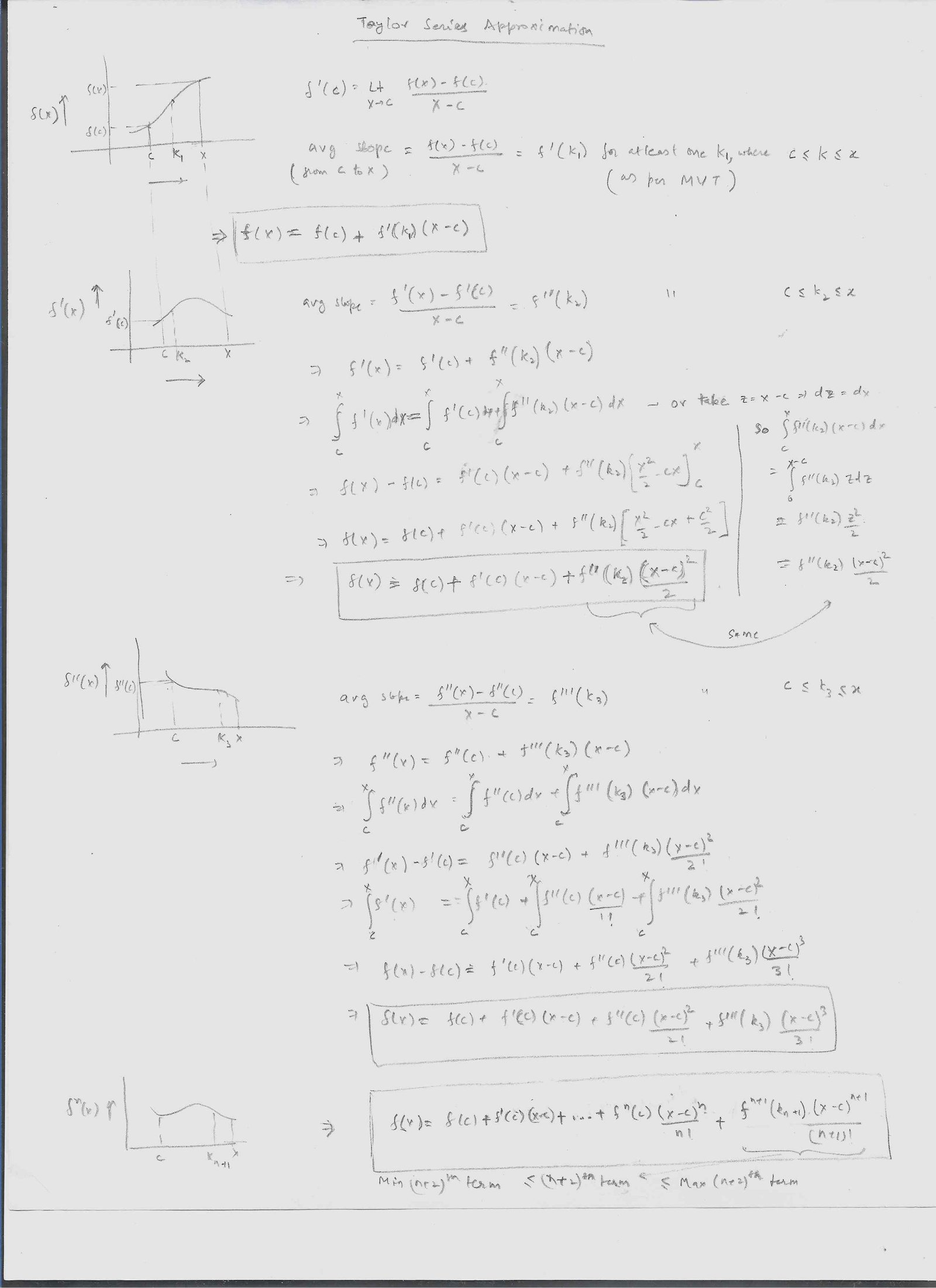
In this alternative proof, we find that for some Kn, the func equals the TS rep exactly with finite terms in it. We use that to prove that a upper bound can be placed.
Lagrange Thm (LT) or Taylor Remainder (TR) Theorem: What we derived above for upper bound on the error is called Lagrange Thm or Taylor Remainder Theorem, Formula is |E(x)| ≤ M*[(x-c)^(N+1)]/(N+1)! . So, for error at x=b, we get |E(b)| ≤ M*[(b-c)^(N+1)]/(N+1)! where M is the max value of |f(N+1)(x)| in the range of x∈[b,c]. To get max error within x∈[a,b], we need to have c within [a,b]. Then max value will be the max of err func at a and b, i.e E(a) with x in the range of x∈[a,c] and E(b) with x in the range of x∈[b,c] .
ex: To get an error < 0.001 for sin(0.4), what's the least degree of poly needed in MS?
E(x) = f(x) - P(x), where f(x)=sin(x). We want E(0.4) < 0.001. f(N+1)(x) = sin(N+1)(x) = cos(x) or sin(x) which is always -1 to 1, i.e M=1. sin(N+1)(x) ≤ 1. So, using LT, |E(b)| ≤ M*[(b-a)^(N+1)]/(N+1)! => |E(0.4)| ≤ 1*[(0.4-0)^(N+1)]/(N+1)! = 0.4^(N+1)]/(N+1)!. if we take N=4, we get 0.4^5/5! = 0.0008 which is < 0.001. So, by taking degree upto 4, we can get error bounded to < 0.001. i.e sin(x) = x − x^3/3! will suffice to give error < 0.001. We can check that: sin(0.4) = 0.38942, while MS gives 0.4-(0.4)^3/3!=0.38933, so error is = 0.38942 - 0.38933 = 0.00009 < 0.001
Region or Interval of convergence (ROC or IOC):
The series obtained above as MS or TS may or may not converge for all values of x. So, we also define a region of convergence (ROC), since outside of this ROC, the series (TS or MS) may not represent the original func at all. The range of values (including both -ve and +ve values) where the infinite series will converge is called IOC or ROC.
Another term Radius of Convergence is also used, which indicates the +ve value or the radius within which the series will converge (excluding the endpoint). Radius of Convergence is 1/2 of the IOC/ROC as it indicates the radius of such range.
We generally use Ratio Test to find out if the series converges or not. Remember that series converging or diverging depends on the value of x.
Parametric Eqn & Polar Coord
Parametric eqn and Polar coord are covered in Calculus, even though are geometry concepts. However, their use is primaily in calculus, so they are introduced here.
Parametric Eqn (PE):
Assume eqn of form x^2 + y = x + y^2 + xy. This eqn can't be written in closed form, but it can be exprssed in another form, by introducing another var "t", and then expressing x and y in terms of t. i.e x=f(t), y=g(t). t is called parameter, and the 2 eqn are called PE. To express y in terms of x, we can eliminate t and substitute. PR also have a direction, and the direction is as "t" increases.
Find dy/dx => To find dy/dx, we can either find it by using eqn of form y=h(x), or we can use dy/dx = (dy/dt) / (dx/dt) [this is true as dy/dx = dy/dt *dt/dx}. This way, we don't have to convert eqn from from parametric form.
Find d2y/dx2 = d/dx (dy/dx)= d/dt (dy/dx) * (dt/dx) = d/dt (dy/dx) / (dx/dt). We already found dy/dx from above, which is in terms of t, so now we need to diferentiate wrt t.
ex: x(t)=2Sin(1+3t), y(t)=2t^3. Find dy/dx. Here, dy/dx= dy/dt / dx/dt = 6t^2 / (6Cos(1+3t))
Arc length in PE: It's similar to how we fund arc length before, except that the eqn is in terms of "t" now. From before, L = b
a∫ √ ( 1 + f’(x)2 ) dx = b
a∫ √ ( 1 + [dy/dt / dx/dt]2 ) dx = b
a∫ √ ( dx/dt + [dy/dt / dx/dt]2 ) dx = b
a∫ √ ( [dx/dt]2 + [dy/dt]2 ) dt/dx * dx = t=d
t=c∫ √ ( [dx/dt]2 + [dy/dt]2 )dt = t=d
t=c∫ √ ( f'(t)2 + g'(t)2) dt . Here limits have changed to be in terms of t and both func are also in terms of t. Easy to solve.
ex: x(t)=Sin(t), y(t)=Cos(t). Find L of arc from t=0 to t=π/2. L = t=π/2
t=0∫ √ ( f'(t)2 + g'(t)2) dt = π/2. This makes sense as The graph is a circle of unit radius, and we are measuring arc of 1/4th of circle which is π/2.
Vector Valued Func: Similar to non vectored func.